Aware Intelligence
An always-on recurrent system in PyTorch that decides from its own internal state when to speak, tested in pre-registered experiments, with a scoring pipeline built for a public anomaly-detection benchmark.
| Core | closed-form continuous-time (CfC) cell, the time step an explicit input |
| Rhythm | Kuramoto oscillator bank in theta, alpha and gamma bands |
| Gate | observer (ignition × uncertainty × phase coherence, amplified by surprise), Schmitt trigger, threshold lowered by arousal |
| Opt-in modules | vector memory, a vision input, a self-model |
| Text readout | byte-level decoder trained on enwik8, 2.28 bits per byte |
| Experiments | E1 to E14, pre-registered from E10 (15 July 2026) |
| Benchmark | TSB-AD-M, scored by VUS-PR with the publisher's own code |
| Stack | PyTorch, PPO, PySide6 and pyqtgraph dashboard, pygame simulation |
Aware Intelligence is a neural system I built from scratch in PyTorch that keeps running between inputs and decides from its own internal state when to emit anything. It is not a language model, and not a claim about consciousness. Between 13 July and 23 September 2026 I tested it in numbered experiments, E1 to E14, and kept a dated log of every decision, prediction and retraction. Its clearest finding came from a health probe I wrote for it: the text checkpoint with the best score had 82.5% of its state neurons stuck at their limits, and the retrained one had none stuck and scored better. On 27 July I moved it to a public anomaly-detection benchmark, under the rule that the scoring pipeline must reproduce published numbers before the system is scored.
A state that keeps moving, and a gate on top of it
The starting idea was a system with activity of its own between inputs, an inner observer, and a balance it returns to after a push. I built the core, which I call the substrate, on 13 July. The state lives in a CfC cell that takes the elapsed time as an input, so it can be stepped at any rate. A bank of Kuramoto oscillators drives it: sweeping the coupling moves their coherence from 0.08 to 0.99, with the transition near K = 2 (E2). With the oscillators and noise switched on, the state keeps changing under zero input (mean step 3.7 × 10⁻²); with them off it settles to 3.0 × 10⁻⁹ (E1). A homeostat pulls an arousal signal back to its set point.
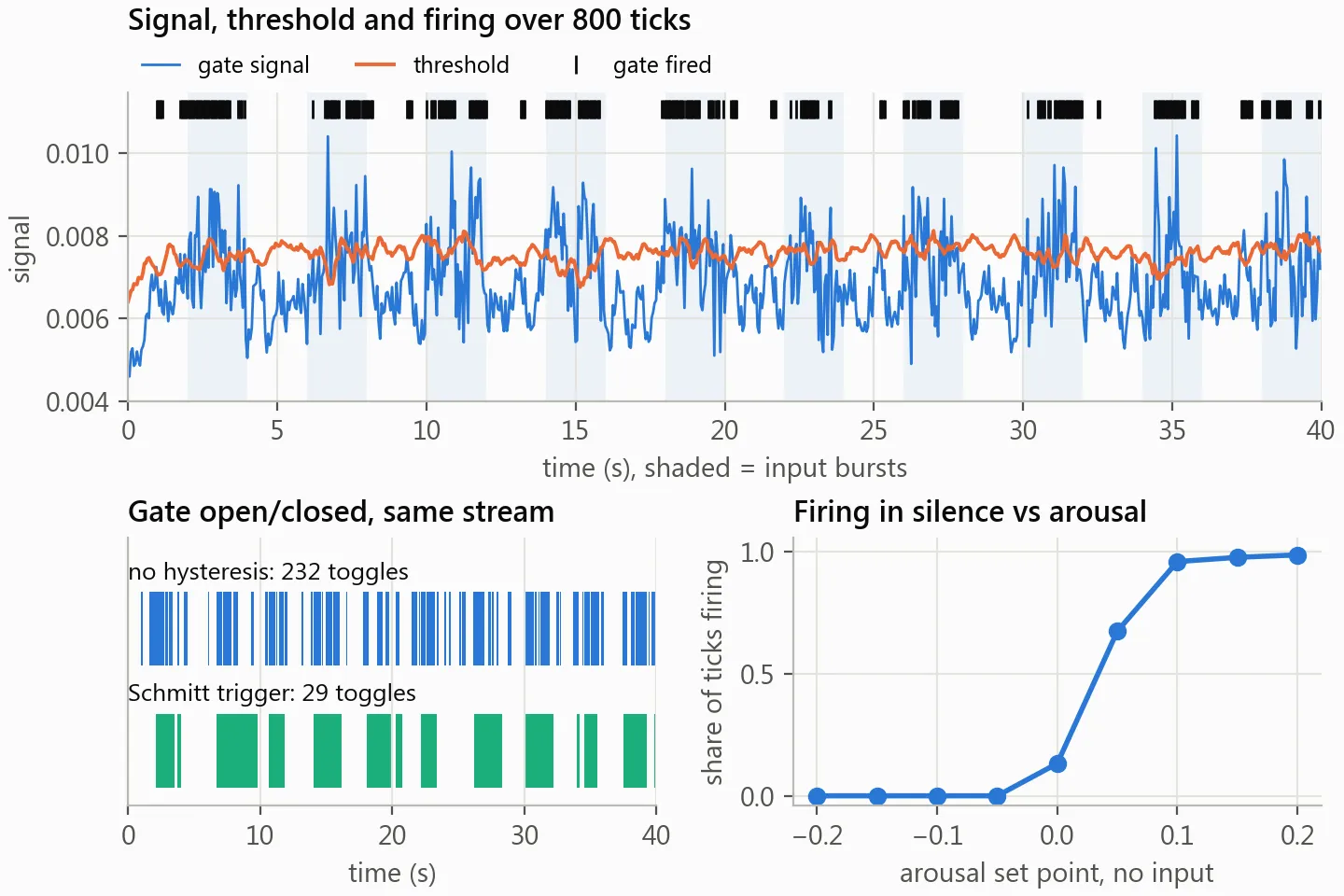
The observer multiplies a workspace-style ignition signal by the model’s own uncertainty and the phase coherence, amplifies it by surprise, the error of a small forward model that predicts the next state from the current one, and fires when the result crosses a threshold that arousal lowers. A Schmitt trigger makes it stop at a lower level than it starts at; over the same input stream that cut the gate’s switching from 232 toggles to 29 (E4).
Three further modules are opt-in and off by default: a vector memory, a vision input and a self-model. With the vector memory, a cue was still recovered with 100% accuracy 40 ticks after it disappeared, against 16% without it (chance 17%, E7). A self-model trained only on the system’s own future predicted whether it would speak on the next tick at AUROC 0.995, against 0.949 for repeating the last tick, and flagged both regime changes in a 1,200-tick run with no false alarms (E9).
A checkpoint that scored well while its state was dead
I trained the core as a byte-level text model on enwik8, and by 14 July the best
checkpoint reached 2.33 bits per byte. Then I wrote a probe that runs the system
headless, injects text at chosen ticks, compares it against an identical twin
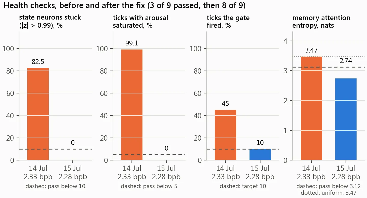
that gets no input, and runs nine pass/fail health checks. It found 82.5% of the
state neurons stuck at their limits even with zero input, arousal saturated on
99.1% of ticks, a gate calibrated for 10% firing at 45%, and a memory attending
to every slot equally. The checkpoint passed 3 of the 9 checks and its speech was
a row of ] characters. Cross-entropy never penalises a saturated unit: a neuron
stuck at its limit is a constant, and a constant is a free bias for the decoder.
The fix came in three parts. A penalty on units near their limits, free below |z| = 0.9 and quadratic above it, removed the stuck neurons under training input, but the arousal signal still saturated the moment the system ran idle. So each training sequence now continues for 32 free-running ticks with no text, and the penalty applies there too, since idle is the state the system spends most of its time in. The gate calibration measures the real firing rate and bisects the threshold toward the target. The retrained checkpoint of 15 July had no neurons stuck, a gate at 10.0% and 8 of 9 checks passed, and its bits per byte improved to 2.28. The check it still fails: an input’s trace in the state halves in about 4 ticks, short of my 10-tick bar.
Pre-registered from E10 onward
From E10 on 15 July, each experiment’s hypotheses and the result that would falsify them went into the log before the run. Several were refuted. Trained to hold a cue for 5 ticks, the memory kept it decodable for about 73 ticks, which refuted my prediction that retention would scale with the trained delay (E10). In a foraging world where food only refuels and the score comes from collecting stars, the agent still ate 18.68 items per 1,000 ticks against 1.48 for a random walk (E11b, 16 July, one seed). After 250 training updates a baseline given a tuned reward for food collected 2.5 times the stars of the homeostatic drive; trained to 1,500 updates, all three variants finished within 9% of each other. The drive’s one lasting effect was internal: it was the only variant whose memory still read from several slots instead of one. At that length 87 to 92% of the state was stuck in every variant, and a saturation penalty ten times the one that had worked in E11, the earlier version where food was the score, did not free it. E12, an economy that puts a price on each question the agent asks, was built and never run.
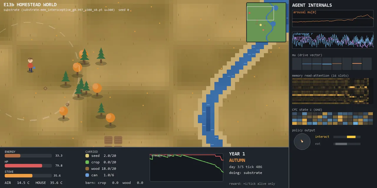
E13 and E13b (17 to 19 July) are a farming survival world with seasons, a house with a wood stove, crops and a barn. The only reward is +1 per tick alive. E13b makes it a continuous map with a river and forest, where the agent moves freely and sees only what is near it. A year is 800 ticks. A random policy lives 0.50 years, a hand-written eat-when-hungry rule 0.77 years before it freezes in the first winter, and a scripted homesteader that stocks the barn almost always reaches the four-year cap.
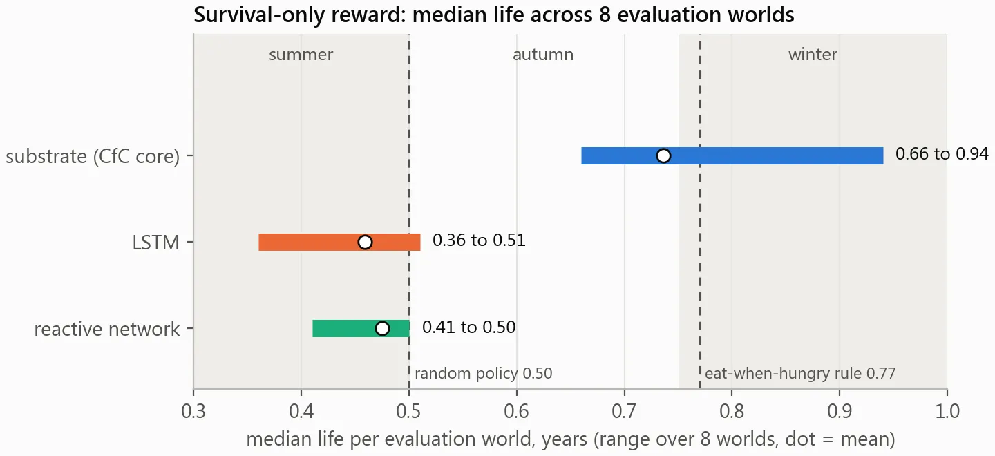
In July I trained the substrate, an LSTM and a reactive network with PPO on the same reward; the two baselines at one learning rate, the substrate at two. Across eight evaluation worlds the substrate’s median life was 0.66 to 0.94 years, against 0.36 to 0.51 for the LSTM and 0.41 to 0.50 for the reactive network, and it won in every world. Both baselines stayed at the random policy’s level of about half a year. In absolute terms the result is modest: the substrate’s mean of 0.74 years sits just under the eat-when-hungry rule, and no trained agent reached a median life of one year, the mark of surviving a first winter that I had set as the bar for a real headline.
One checkpoint, after 300 updates, chopped and stored wood in autumn at 11.32 times its rate in the other seasons, which I first read as preparing for winter. Re-run over three training seeds and eight worlds, 22 of the 24 evaluations gave no reading at all, because the ratio needs time in every season and agents at 300 updates rarely lived into winter; the two that did gave 11.32 and 0.95. The metric was measuring survival, and I withdrew the claim on 19 July. The same re-run showed that a fixed checkpoint’s median life varies from world to world by a coefficient of variation of 12 to 22%, more than the 9% learning-rate gain I had reported the day before from a single world. Paired by training seed and world, the substrate’s lower learning rate still won 19 of 24 comparisons, by 30% on average (one-sided sign test, p = 0.003), and replacing the linear value head with a small MLP added another 10% (18 of 24, p = 0.011).
On 21 July I fixed a trainer bug that had cut backpropagation through time for every agent in the batch whenever one of them died. It handicapped both recurrent networks, the substrate and the LSTM, in all of the runs above. On 7 October I repeated the comparison with the fix: all three networks at the same two learning rates, three training seeds each, tested in eight worlds none of them had trained or been selected in. The result reversed. The reactive network, which has no memory, lived 0.62 years on average, the LSTM 0.56 and the substrate 0.50, level with a random policy at 0.49. Paired by training seed and world, the substrate won 6 of 24 comparisons against the reactive network and 8 of 24 against the LSTM (one-sided sign test, p = 0.997 and 0.968). The July checkpoint still lives 0.70 years in those eight worlds; training the same design again did not reproduce it. Under the outcome rules I wrote down before the run, the survival claim does not hold, and I withdrew it.
Moving to a benchmark someone else wrote
Every number up to then came from worlds and scorers I had written, and the best replicated result of the survival line, the MLP value head, was a fact about PPO rather than about the system. On 27 July I froze the survival line and registered E14: the observer gate as an alerting policy for streaming data, scored on TSB-AD-M, a public multivariate anomaly-detection benchmark, with the publisher’s scoring code running in its own pinned Python environment. The oscillators have no registered role in this track.
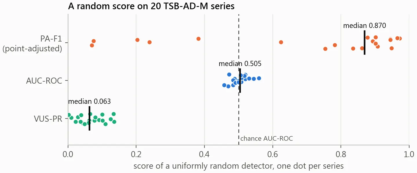
The pipeline had to pass two checks before the system was allowed a number. Gate A (28 July) reproduced a known flaw in the field’s common point-adjust protocol: on 20 real series a random score reaches a median PA-F1 of 0.870 while its median AUC-ROC stays at chance, 0.505. That effect is pinned as a unit test. Gate B re-runs a published baseline. TSB-AD’s reference PCA does not fit this machine: on one 200,001 × 19 series it reached 21.8 GB of memory and had not finished after 31 minutes. KMeansAD does. Under a rule set on 29 July its mean was not compared with the published one before all 180 evaluation series were in; on 7 October it finished all 180 with a mean VUS-PR of 0.2924 against the published 0.2949, 0.9% apart, and Gate B passed.
The hypotheses are registered. The system must reach VUS-PR 0.3066, the published score of LSTMAD, the method closest to it in architecture, which would place it 8th of 30 on the community leaderboard (tied with a cluster at 0.31); below 0.2950, AutoEncoder’s published score, it is registered as a failure, and a score in between as a miss. At the same alert budget, the gate must catch more of the anomalies, and catch them sooner, than a fixed threshold on the same score, and since 23 September also than the same Schmitt trigger applied to the raw surprise score, so that a win cannot come from hysteresis alone.
The scoring path is fixed in advance as well: only the forecasting head trains, on the same clean opening stretch of each series that the published baselines fit on, while the core stays at its random initialisation. The adapter that runs the system on the benchmark was not written by 23 September, so the system itself has no score on it.